This page was generated from /home/docs/checkouts/readthedocs.org/user_builds/blm/checkouts/latest/docs/tasks/task4.ipynb. Interactive online version: Slideshow:

1.5. Understanding Surface Properties (4): Heat Storage and Surface Resistance

1.5.1. Objectives

1. Understand how to calculate ground heat flux.

2. Understand how to back-calculate surface resistance.

1.5.2. Calculation of heat storage: OHM (Objective Hysteresis Model) and a simple scheme

The objective hysteresis model helps us estimate the ground surface heat flux using the measured net radiation data. The equation for this model is as follows:

\[\Delta Q_{S}=a_{1} Q^{*}+a_{2} \frac{\partial Q^{*}}{\partial t}+a_{3}\]

where \(\Delta Q_S\) is the ground heat flux (W m\(^{-2}\)), \(Q^*\) is the net radiation (W m\(^{-2}\)), and \(a_{1-3}\) are the coefficients to be determined from measurements

In this task, we focus on a simpler model instead of the above question using just the first term:

\[\Delta Q_{S}=a_{1} Q^{*}\]

The aim is to find \(a_1\) using the measurements.

1.5.2.1. Tasks

1.5.2.1.1. Load necessary packages

import numpy as np
import matplotlib.pyplot as plt
import pandas as pd
from pathlib import Path

1.5.2.1.2. Loading data

group_number = 7
path_dir = Path.cwd() / 'data' / f'{group_number}'
# examine available files in your folder
list(path_dir.glob('*gz'))

[PosixPath('/Users/hamidrezaomidvar/Desktop/BLM-task4/data/7/US-Whs_clean.csv.gz'),
 PosixPath('/Users/hamidrezaomidvar/Desktop/BLM-task4/data/7/US-NC1_clean.csv.gz')]

# specify the site name
name_of_site = 'US-Whs'

# load dataset
site_file = name_of_site + '_clean.csv.gz'
path_data = path_dir / site_file
df_data = pd.read_csv(path_data, index_col='time', parse_dates=['time'])
df_data.head()

	WS	RH	TA	PA	WD	P	SWIN	LWIN	SWOUT	LWOUT	NETRAD	H	LE	USTAR	ZL
time
2007-06-29 13:30:00	4.063	12.6475	34.790	86.3667	273.75	0.0	1096.50	NaN	NaN	NaN	609.9	339.3645	12.2582	0.4036	NaN
2007-06-29 14:00:00	3.636	12.2413	35.140	86.3323	322.30	0.0	1057.00	NaN	NaN	NaN	562.8	290.9766	14.5989	0.5052	NaN
2007-06-29 14:30:00	3.107	12.0811	35.490	86.3048	316.75	0.0	1107.50	NaN	NaN	NaN	596.4	359.2087	16.1474	0.3566	NaN
2007-06-29 15:00:00	4.302	11.6801	36.190	86.2589	292.30	0.0	1108.00	NaN	NaN	NaN	613.5	360.5630	10.0565	0.5340	NaN
2007-06-29 15:30:00	3.676	13.7432	34.785	86.2429	209.20	0.0	496.15	NaN	NaN	NaN	232.0	200.0689	64.8520	0.4503	NaN

Assuming surface energy closure in measurements is perfect, i.e., \(Q^*=Q_H+Q_E+\Delta Q_S\)

Note: conduct the derivation at different sites separately so you can get two sets of coefficients for later comparison.

1.5.2.1.3. Calculating \(\Delta Q_S\)

df=df_data.filter(['NETRAD','H','LE'])
df.dropna(inplace=True)
QSTAR=df.NETRAD
QH=df.H
QE=df.LE

QS=QSTAR-QH-QE


QS.plot(figsize=(15,4))
plt.ylabel('$\Delta Q_S$')

Text(0, 0.5, '$\\Delta Q_S$')

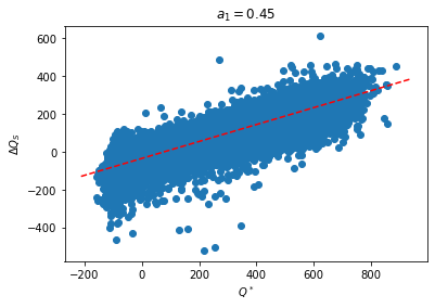
1.5.2.1.4. Finding \(a_1\)

from scipy.stats import linregress

fig, ax = plt.subplots(1, 1)
slope = linregress(QSTAR, QS).slope
intercept=linregress(QSTAR, QS).intercept

ax.scatter(QSTAR, QS)
lim = ax.get_xlim()
plt.plot(lim, [x * slope+intercept for x in lim], color='r', linestyle='--')
plt.title(f'$a_1 = {slope:.2f}$')
plt.ylabel('$\Delta Q_S$')
plt.xlabel('$Q^*$')

Text(0.5, 0, '$Q^*$')

1.5.2.1.5. Compare derived OHM coefficients between sites

# your code here

1.5.2.1.6. Calculate \(\Delta Q_S\) using provided OHM coefficients

Use the values provided in this page of SUEWS manual

# your code here

1.5.2.1.7. examine the SEB closure using calculated

Think about proper metrics for quantitative examination.

# your code here

1.5.3. calculate surface resistances \(r_s\)

\(r_s\) can be calculated as following

\[r_{s}=\left(\frac{s \beta}{\gamma}-1\right) r_{a}+\frac{C_{a} V}{\gamma Q_{E}}\]

where

\[\beta=\frac{Q_{H}}{Q_{E}}\]

\[C_{a}=\rho c_{p}\]

\[V=e_{s}-e_{a}\]

\[\gamma = \text{psychrometric constant}\]

\[s=\text{slope of saturation evaporation pressure curve vs air temperature}\]

We are going to calculate each part separately and eventually integrate all parts together to get \(r_s\)

1.5.3.1. Calculate \(r_a\)

You should calculate \(r_a\) using task 3 and the function that you implemented before for the site: similarly for \(z_0\) and \(d\).

# your code here

1.5.3.2. Calculating \(\beta=\frac{Q_{H}}{Q_{E}}\)

df_val = df_data.loc[:, ['LE','H', 'USTAR', 'TA', 'RH', 'PA', 'WS']].dropna()

# your code here

1.5.3.3. Calculating \(C_{a}=\rho c_{p}\)

For this, you can use the available functions in utility.py

Important:

In these functions, pressure is in hPa; so you need to convert the pressure from kPa to hPa

df_val.PA *=10

from utility import cal_dens_air, cal_cpa

#rho = cal_dens_air(Press_hPa, Temp_C)  #use this to calculate rho
#cp = cal_cpa(Temp_C, RH_pct, Press_hPa) #use this to calculate cp

1.5.3.4. Calculating \(s\)

# This package is needed
!pip install atmosp

from utility import cal_des_dta
# s = cal_des_dta(Temp_C, Press_hpa) #use this to calculate s

1.5.3.5. Calculating \(V=e_{s}-e_{a}\)

from utility import cal_vpd
# V = cal_vpd(Temp_C, RH_pct, Press_hPa)  #use this to calculate V

1.5.3.6. Calculating \(\gamma\)

from utility import cal_gamma
#gamma = cal_gamma(Press_hPa) #use this to calculate gamma

1.5.3.7. Integrate: calculate \(r_s\)

# your code here