Note

Please report issues or ask questions about this site on the GitHub page.

10. Eddy Covariance

10.1. Sonic Anemometer

A sonic anemometer derives the wind-speed from transit times of acoustic pulses travelling in both directions along a fixed path. The wind-speed component along the path is proportional to the difference between the transit times. Three sets of transducer pairs are used to derive the three components of the wind vector u, v, w. In addition, the speed of sound can be deduced:

(10.1)\[c^2=403T_s,\]

where \(T_s\) is the sonic temperature:

(10.2)\[T_s=T(1+0.32 e/p)\]

where \(T\) is the dry bulb temperature, \(e\) is the water vapour pressure, and \(p\) is the air pressure. The sonic temperature is approximately equal to the virtual temperature \(T_v\).

In practical use, the covariance: \(\overline{w^{\prime} T_{s}^{\prime}} \approx \overline{w^{\prime} T^{\prime}}\) and therefore the sonic anemometer can be used to estimate turbulent sensible heat flux (\(Q_H\)). Sonic anemometers are the standard instrument used to observe turbulence in the atmospheric boundary layer.

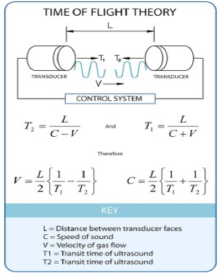
Fig. 10.1 Principle behind sonic measurement of velocity and speed of sound

10.2. Infra-red Gas Analyser (IRGA)

IRGA allows measurement of variations in water vapour and carbon dioxide allowing the latent heat flux and carbon dioxide to be measured. The specific humidity of water vapour \(q\) is expressed in units of kg kg^-1. The absolute humidity (kg m^-3) is derived by taking the molecular weight of water into account (1 mol = 18 g = 0.018 kg) and similarly for carbon dioxide concentrations (molar mass 44 g mol^-1).

1. Open-path IRGA: Measurements are made at station pressure.

2. Closed-path IRGA: Air is sucked down a tube into the instrument itself

Fig. 10.2 Schematic of the LI-COR Li 7500 open path infra-red gas analyser (IRGA) (source: LI-COR)

10.2.1. Instruments at Different Sites

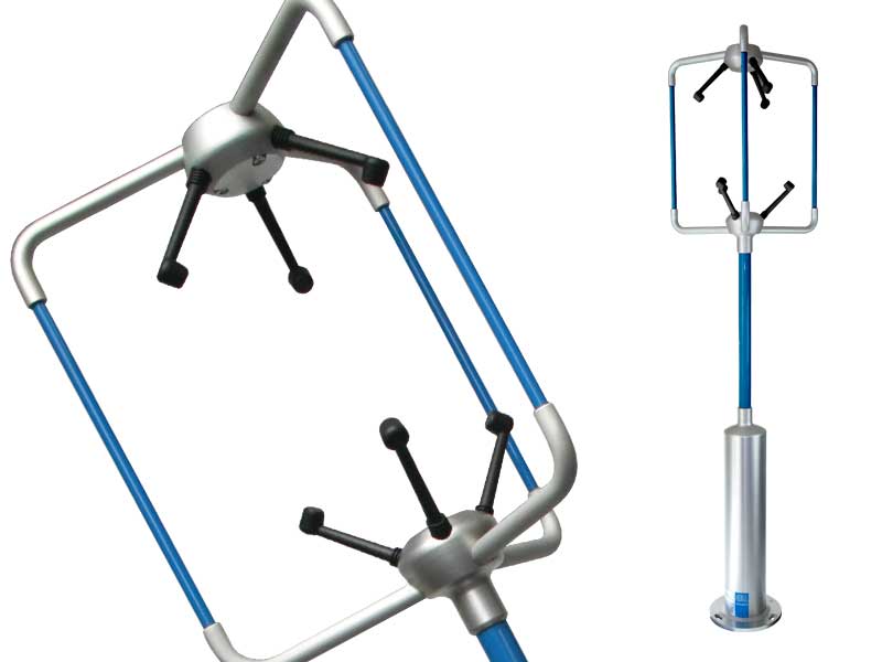
Fig. 10.3 Gill R3 sonic anemometer (source: Gill Instruments).

1. Site: URAO

   • see Observatory.

2. Site: AmeriFlux

   • Each site has a key reference that gives the details of the instruments used.

   • Please see AmeriFlux Site page for details (login required with free registration).

10.3. Eddy covariance (EC) method to measure fluxes

Note

\(\tau\) unfortunately (by convention) is used for both momentum and time lag

EC is regarded as the standard method to measure fluxes as it quantifies directly the contribution by each eddy. EC fluxes of momentum, heat and moisture require fast response (10-20 Hz) measurements to capture the scales of turbulence contributing to fluxes. The momentum flux (or Reynolds stress) is calculated from:

(10.3)\[\tau=\rho \sqrt{\left(\overline{u^{\prime} w^{\prime}}^2 +\overline{v^{\prime} w^{\prime}}^2\right)}\]

This considers any vertical transfer of lateral momentum \(\overline{u^{\prime} w^{\prime}}\). The sensible heat flux is given by:

(10.4)\[Q_{H}=\rho c_{p} \overline{w^{\prime} T^{\prime}}\]

assuming that \(T\approx \theta\) , and the latent heat flux (\(Q_E\) ) is given by:

(10.5)\[Q_{E}=L_{V} \overline{w^{\prime}} q^{\prime}\]

where \(L_{V}\) is the latent heat of vaporisation (\(\approx 2.45 \times 10^6 \text{kg}^{-1}\)) and q is the specific humidity. These equations assume the vertical component of the flux dominates, i.e. flow is homogeneous and steady.

10.4. Rotation of EC data

In theory, the wind component u is defined as being aligned with the mean wind direction, and thus the mean vertical component. The instrument itself has a fixed frame of reference, so how is this achieved? The frame of reference is rotated to align the new u axis with the measured mean wind vector.

This is called double rotation as it is usually done in two steps:

1. rotate through angle \(\alpha\) around the vertical axis so that;

2. rotate through angle \(\beta\) around the lateral axis so that.

Mathematically this is given by:

(10.6)\[\begin{split}\begin{aligned} \left[ \begin{array}{c}{u_{2}} \\ {v_{2}} \\ {w_{2}}\end{array} \right]= \left[ \begin{array}{ccc}{\cos \alpha \cos \beta} & {\sin \alpha \cos \beta} & {\sin \beta} \\ {-\sin \alpha} & {\cos \alpha} & {0} \\ {-\cos \alpha \sin \beta} & {-\sin \alpha \sin \beta} & {\cos \beta}\end{array}\right] \times \left[\begin{array}{c} {\overline{u}} \\ {\overline{v}} \\ {\overline{w}} \end{array} \right] \end{aligned}\end{split}\]

where \(\alpha=\tan ^{-1}(\overline{v} / \overline{u})\) and \(\beta=\tan ^{-1}(\overline{w} / \sqrt{\overline{u}^{2}+\overline{v}^{2}})\).

10.5. Co-ordinate transformation of wind components

It is not generally possible to mount a 3-directional anemometer so that its axes coincide with the directions \(\overline{u}>0, \overline{v}=0, \overline{w}=0\) (where the over-bar denotes time-averaging over many data values). However, a co-ordinate transformation applied to the sensed components \(U, V, W\) means that the transformed component series \(u, v, w\) satisfies the above properties. The transformed components can be calculated using

(10.7)\[\begin{split}\begin{aligned} \begin{array}{l} {u=U \cos A \cos B+V \cos A \sin B+w \sin A} \\ {v=V \cos B-U \sin B} \\ {w=W \cos A-U \sin A \cos B-V \sin A \sin B} \end{array} \end{aligned}\end{split}\]

where angle \(A=\arctan{(\overline{W}/S)}\), \(\sin B=\overline{V}/S\), \(\sin B=\overline{U}/S\) , \(S=\overline{U}^2+\overline{V}^2\).

10.6. Errors in statistics

Reynolds averaging requires separation into a mean part (low frequency variation) and fluctuations (high frequency) from which we calculate covariances, variances, etc which are all in some sense a mean value taken over many samples. Usually we calculate the standard error of a mean.

(10.8)\[\Delta_{\alpha} = \sigma_{\alpha}/\sqrt{N}\]

where \(N\) is the number of samples taken. In turbulence, we know that each discrete measurement – or sample – is not fully independent of the last one, and the number of samples which are correlated is determined by the integral time-scale LT. So N should be replaced by the number of independent samples:

(10.9)\[N_{i} = T/L_{T}\]

where \(T\) is the period over which data is being averaged.

Statistical stationarity of a time series means that variances and covariances approach a stable value as the averaging time is extended, and the errors associated get smaller. So how long is long enough? The aim is to have a large number of samples.

So given that the averaging period \(T = N\Delta t\), there is a trade-off between the sampling period and the interval between samples, \(\Delta t\). If \(\Delta t\) is too long, then \(T\) must be increased to keep \(N\) large. The danger is that T is too long, and the statistics are no longer stationary, i.e. the turbulent flow has changed in response to external factors like a gust front passing through. Typically, sampling rate is 10-20 Hz, and the averaging period is 30-60 minutes depending on conditions.

10.7. The autocorrelation function and integral timescale

As well as calculating the covariance between two variables, it is instructive to look at the auto-correlation function, or the correlation of a variable with itself at later time-steps. For instance, consider the u component of the wind

(10.10)\[R_{u}(\tau) = \frac{\overline{u^{'}(t)u^{'}(t + \tau)}}{{\sigma_{u}}^{2}}\]

Hence \(R(\tau)=1\) at \(\tau = 0\). The rate at which \(R(\tau)\) decreases with lag is related to the size distribution of eddies. Large eddies cause slower variations in the time series, and thus the auto-correlation will decrease more slowly with lag than for a time series dominated by smaller eddies. Hence, a simple measure of ‘typical eddy size’ is given by the integral timescale \(L_T\) , defined as

(10.11)\[L_{T} = \int_{0}^{\infty}{R(\tau)\text{dτ}}\]

From Taylor’s frozen turbulence hypothesis, the integral length-scale \(L_X =\overline{u}L_T\). The integral length-scale for a variable can be thought of as the decorrelation length-scale, i.e. for two sensors separated beyond this distance, the turbulence measured at each will not be correlated.

10.8. Calculation of errors on covariances

For a covariance (e.g. \(\overline{w'T'})\ \) the error can be calculated: As \(\overline{w'T'}\) is a mean of a large number of quantities, we might expect its standard error to be given by:

(10.12)\[\Delta\overline{T^{'}w^{'}} = \sigma(T^{'}w^{'})/\sqrt{N_{i}}\]

where \(\sigma(T^{'}w^{'})\) is the standard deviation of \(\sigma(T^{'}w^{'})\) and Ni is the number of independent samples. Assuming all samples are independent of each other, estimate the standard error \(\Delta\overline{T^{'}w^{'}}\). Is this likely to be an accurate estimate? The number of independent samples is more accurately given by:

(10.13)\[N_{i} = N\frac{\Delta t}{L_{t}},\]

where \(N\) is the total number of samples, \(\Delta t\) is the time between samples and \(L_t\), is the integral timescale for the time series of \(T^{'}w^{'}\). To estimate the integral timescale, we need to calculate and plot the autocorrelation function for \(T^{'}w^{'}\), and read off the time at which it falls to \(1/e = 0.368\).