This page was generated from /home/docs/checkouts/readthedocs.org/user_builds/blm/checkouts/latest/docs/tasks/task2-1.ipynb. Interactive online version: Slideshow:

1.3. Understanding Surface Properties (2): LAI

1.3.1. Objectives

1. Understand the dynamics of LAI at different temporal scales (e.g., sub-daily, seasonal)

2. Understand the effects of LAI dynamics on albedo

1.3.2. Tasks

1.3.2.1. load necessary packages

import pandas as pd
import numpy as np
import matplotlib.pyplot as plt
from datetime import datetime
from pathlib import Path
import datetime

1.3.2.2. Name of the site and group number

1.3.2.3. loading data for albedo calculation

group_number=2
path_dir = Path.cwd()/'data'/f'{group_number}'
# examine available files in your folder
list(path_dir.glob('*gz'))

[PosixPath('/Users/hamidrezaomidvar/Desktop/BLM/docs/tasks/data/2/US-MMS_clean.csv.gz')]

name_of_site='US-MMS' #

# load dataset
site_file=name_of_site+'_clean.csv.gz'
path_data = path_dir/site_file
df_data = pd.read_csv(path_data, index_col='time',parse_dates=['time'])
df_data.head()

	WS	RH	TA	PA	WD	P	SWIN	LWIN	SWOUT	LWOUT	NETRAD	H	LE
time
1999-01-01 01:00:00	2.98	NaN	NaN	99.0	95.50	0.0	0.0	190.0	0.0	250.7	-60.7	-21.310	-0.350
1999-01-01 02:00:00	2.93	NaN	NaN	99.0	108.71	0.0	0.0	188.0	0.0	248.8	-60.8	-14.473	-0.321
1999-01-01 03:00:00	2.96	NaN	NaN	99.0	122.46	0.0	0.0	187.5	0.0	247.6	-60.1	-16.784	-0.786
1999-01-01 04:00:00	3.03	NaN	NaN	99.1	118.99	0.0	0.0	187.6	0.0	247.7	-60.1	-12.367	-0.191
1999-01-01 05:00:00	3.63	NaN	NaN	99.2	124.80	0.0	0.0	186.4	0.0	246.9	-60.5	-23.069	-0.650

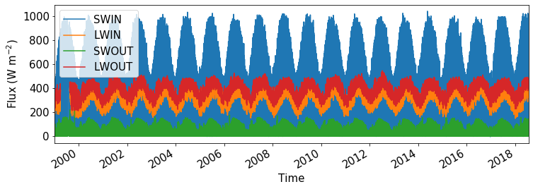
1.3.2.4. Take a look at the raditation data

fontsize=15
df_data.loc[:,['SWIN','LWIN','SWOUT','LWOUT']].plot(figsize=(12,4),fontsize=fontsize)
plt.ylabel('Flux (W m$^{-2}$)',fontsize=fontsize)
plt.xlabel('Time',fontsize=fontsize)

Text(0.5, 0, 'Time')

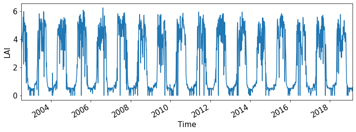
1.3.2.5. Loading LAI data + some data cleaning

def DOY_to_datetime(row):
    year=int(row['modis_date'][1:5])
    DOY=int(row['modis_date'][5:])
    return datetime.datetime(year, 1, 1) + datetime.timedelta(DOY - 1)

df_LAI=pd.read_csv('data/MODIS_LAI_AmeriFlux/statistics_Lai_500m-'+name_of_site+'.csv')
df_LAI.columns=['product']+[i.split(' ')[1] for i in df_LAI.columns if i!='product']
df_LAI=df_LAI.filter(['modis_date','value_mean'])


df_LAI.set_index(df_LAI.apply(DOY_to_datetime,axis=1),inplace=True)
df_LAI.drop('modis_date',axis=1,inplace=True)
df_LAI.head()

	value_mean
2002-07-04	5.1042
2002-07-08	3.2211
2002-07-12	3.6012
2002-07-16	4.2047
2002-07-20	4.0568

fontsize=15
df_LAI.plot(legend=False,figsize=(12,4),fontsize=fontsize)
plt.ylabel('LAI',fontsize=fontsize)
plt.xlabel('Time',fontsize=fontsize)

Text(0.5, 0, 'Time')

1.3.3. examine results

1.3.3.1. Choose the desire period

start_period='2006-01-01'
end_period='2007-01-01'

df_data_period=df_data.loc[start_period:end_period]
df_LAI_period=df_LAI.loc[start_period:end_period]

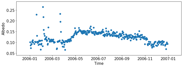
1.3.3.2. Alebdo calculation

ser_alb=df_data_period['SWOUT']/df_data_period['SWIN']
ser_alb=ser_alb[ser_alb.index.time==datetime.time(12, 0)]
ser_alb_clean=ser_alb[ser_alb.between(0,1)&(df_data_period['SWIN']>5)]


plt.rcParams.update({'font.size': 15})
plt.figure(figsize=(12,4))
plt.scatter(ser_alb_clean.index,ser_alb_clean)
plt.ylabel('Albedo')
plt.xlabel('Time')

Text(0.5, 0, 'Time')

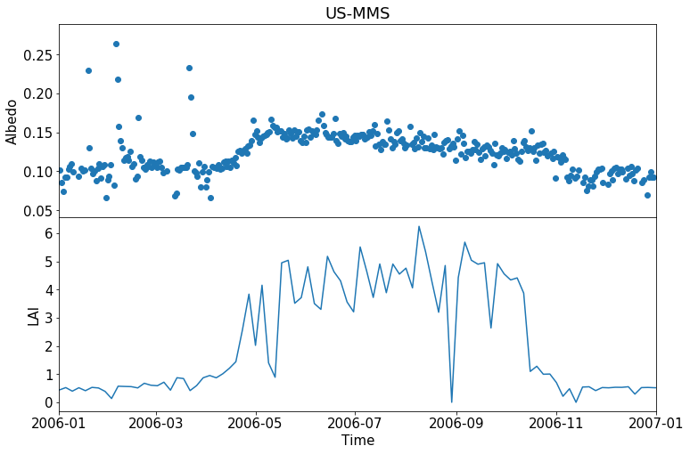
1.3.3.3. explore the relationship between albedo and LAI

plt.rcParams.update({'font.size': 15})
fig,axs=plt.subplots(2,1,figsize=(12,8))
fig.subplots_adjust(hspace=0)
ax1=axs[0]
ax2=axs[1]

ax1.scatter(ser_alb_clean.index,ser_alb_clean)
ax1.set_ylabel('Albedo')
ax1.set_xlim([start_period,end_period])
ax1.set_xticks([])
ax1.set_title(name_of_site)


ax2.plot(df_LAI_period.index,df_LAI_period)
ax2.set_ylabel('LAI')
ax2.set_xlabel('Time')
ax2.set_xlim([start_period,end_period])

(732312.0, 732677.0)