This page was generated from /home/docs/checkouts/readthedocs.org/user_builds/blm/checkouts/latest/docs/tasks/task3.ipynb. Interactive online version: Slideshow:

1.4. Understanding Surface Properties (3): Surface Roughness¶

1.4.1. Objectives¶

Understand how to quantify surface roughness
Understand variability of surface roughness

Tips:

Eddy Covariance observations allow several important parameters to be determined:

Zero plane displacement length \(d\) can be calculated based on vegetation height (think about changes in LAI and porosity). If there is a profile of anemometers (e.g. as at the Observatory) then this can be calculated using that.
Roughness length \(z_0\) can be calculated from the EC data (EddyCovariance) by rearranging the logarithmic law from the neutral wind profile WindProfile).

Do these vary with season? Wind Direction? Create a graph to analyse the data (think about wind directions).
How do these values compare to the literature?
Calculate the aerodynamic resistance \(r_a\).
For scientific background see Roughness and Reading List

1.4.2. Tasks¶

1.4.2.1. load necessary packages¶

[1]:

import numpy as np
import matplotlib.pyplot as plt
import pandas as pd
from pathlib import Path

1.4.2.2. loading data¶

[2]:

group_number = 10
path_dir = Path.cwd() / 'data' / f'{group_number}'
# examine available files in your folder
list(path_dir.glob('*gz'))

[2]:

[PosixPath('/Users/sunt05/Dropbox/6.Repos/BLM-task3/data/10/US-Oho_clean.csv.gz'),
 PosixPath('/Users/sunt05/Dropbox/6.Repos/BLM-task3/data/10/CA-TPD_clean.csv.gz')]

[3]:

# specify the site name
name_of_site = 'CA-TPD'

[4]:

# load measurement heights
df_zmeas = pd.read_csv('data/measurement_height.csv', index_col=0)
df_zmeas.loc[name_of_site].iloc[:]

[4]:

	Variable	Start_Date	Height	Instrument_Model	Instrument_Model2	Comment	BASE_Version
Site_ID
CA-TPD	CO2_1_1_1	2012.0	35.70	GA_CP-LI-COR LI-7200	NaN	LI-7200 IRGA)	02-May
CA-TPD	CO2_1_2_1	2012.0	16.00	GA_SR-LI-COR LI-820	NaN	LI820_CO2_Cnpy_16m (ppm); CO2	02-May
CA-TPD	FC	2012.0	35.70	GA_CP-LI-COR LI-7200	NaN	NaN	02-May
CA-TPD	FH2O	2012.0	NaN	NaN	NaN	NaN	02-May
CA-TPD	LE	2012.0	35.70	GA_CP-LI-COR LI-7200	NaN	NaN	02-May
CA-TPD	PPFD_IN_PI_F_1_1_1	2012.0	35.13	RAD-PAR Quantum	NaN	NaN	02-May
CA-TPD	P_CUM	2012.0	2.00	NaN	NaN	NaN	02-May
CA-TPD	PA_PI_F	2012.0	2.00	NaN	NaN	NaN	02-May
CA-TPD	G_1_1_1	2012.0	0.00	SOIL_H-Plate	NaN	NaN	02-May
CA-TPD	G_2_2_1	2012.0	-0.03	SOIL_H-Plate	NaN	NaN	02-May
CA-TPD	G_3_2_1	2012.0	-0.03	SOIL_H-Plate	NaN	NaN	02-May
CA-TPD	G_4_2_1	2012.0	-0.03	SOIL_H-Plate	NaN	NaN	02-May
CA-TPD	G_1_2_1	2012.0	-0.03	SOIL_H-Plate	NaN	NaN	02-May
CA-TPD	GPP_PI_F	2012.0	35.70	GA_CP-LI-COR LI-7200	NaN	NaN	02-May
CA-TPD	H	2012.0	35.70	GA_CP-LI-COR LI-7200	NaN	NaN	02-May
CA-TPD	H_PI_F	2012.0	35.70	GA_CP-LI-COR LI-7200	NaN	NaN	02-May
CA-TPD	LE_PI_F	2012.0	35.70	GA_CP-LI-COR LI-7200	NaN	NaN	02-May
CA-TPD	NEE_PI	2012.0	35.70	GA_CP-LI-COR LI-7200	NaN	NaN	02-May
CA-TPD	NEE_PI_F	2012.0	35.70	GA_CP-LI-COR LI-7200	NaN	NaN	02-May
CA-TPD	PPFD_IN_1_1_1	2012.0	35.13	RAD-PAR Quantum	NaN	Kipp and Zonen	02-May
CA-TPD	PPFD_IN_1_2_1	2012.0	2.00	RAD-PAR Quantum	NaN	NaN	02-May
CA-TPD	PPFD_OUT	2012.0	35.13	RAD-PAR Quantum	NaN	Kipp and Zonen	02-May
CA-TPD	P	2012.0	2.00	PREC-TipBucGauge	NaN	CSI (heated and Alter Shielded) in a forest op...	02-May
CA-TPD	PA	2012.0	2.00	PRES-ElectBar	NaN	Young Co	02-May
CA-TPD	RECO_PI_F	2012.0	35.70	GA_CP-LI-COR LI-7200	NaN	NaN	02-May
CA-TPD	SW_IN	2012.0	35.50	RAD-Pyrrad-SW+LW	NaN	Kipp & Zonen CNR4	02-May
CA-TPD	SW_IN_PI_F	2012.0	35.50	RAD-Pyrrad-SW+LW	NaN	CNR1_GlobalShortwaveRad_AbvCnpy_36m (W/m2); Ga...	02-May
CA-TPD	LW_IN	2012.0	35.50	RAD-Pyrrad-SW+LW	NaN	Kipp & Zonen CNR4 Net Radiometer	02-May
CA-TPD	LW_OUT	2012.0	35.50	RAD-Pyrrad-SW+LW	NaN	Kipp & Zonen CNR4 Net Radiometer	02-May
CA-TPD	SW_OUT	2012.0	35.50	RAD-Pyrrad-SW+LW	NaN	Kipp & Zonen CNR4 Net Radiometer	02-May
...	...	...	...	...	...	...	...
CA-TPD	SWC_2_1_1	2012.0	-0.02	SWC-TDR	NaN	NaN	02-May
CA-TPD	SWC_2_3_1	2012.0	-0.10	SWC-TDR	NaN	NaN	02-May
CA-TPD	SWC_2_6_1	2012.0	-1.00	SWC-TDR	NaN	NaN	02-May
CA-TPD	SWC_2_4_1	2012.0	-0.20	SWC-TDR	NaN	NaN	02-May
CA-TPD	SWC_2_2_1	2012.0	-0.05	SWC-TDR	NaN	NaN	02-May
CA-TPD	SWC_2_5_1	2012.0	-0.50	SWC-TDR	NaN	NaN	02-May
CA-TPD	SWC_1_3_1	2012.0	-0.10	SWC-TDR	NaN	NaN	02-May
CA-TPD	SWC_1_6_1	2012.0	-1.00	SWC-TDR	NaN	NaN	02-May
CA-TPD	SWC_1_4_1	2012.0	-0.20	SWC-TDR	NaN	NaN	02-May
CA-TPD	SWC_1_2_1	2012.0	-0.05	SWC-TDR	NaN	NaN	02-May
CA-TPD	SWC_1_5_1	2012.0	-0.50	SWC-TDR	NaN	NaN	02-May
CA-TPD	TS_2_3_1	2012.0	-0.10	TEMP-ElectResis	NaN	NaN	02-May
CA-TPD	TS_2_6_1	2012.0	-1.00	TEMP-ElectResis	NaN	NaN	02-May
CA-TPD	TS_2_4_1	2012.0	-0.20	TEMP-ElectResis	NaN	NaN	02-May
CA-TPD	TA	2012.0	36.60	TEMP-ElectResis	NaN	Campbell Scientific Inc (CSI)	02-May
CA-TPD	TS_2_2_1	2012.0	-0.05	TEMP-ElectResis	NaN	NaN	02-May
CA-TPD	TS_2_5_1	2012.0	-0.50	TEMP-ElectResis	NaN	NaN	02-May
CA-TPD	TS_1_3_1	2012.0	-0.10	TEMP-ElectResis	NaN	NaN	02-May
CA-TPD	TS_1_6_1	2012.0	-1.00	TEMP-ElectResis	NaN	NaN	02-May
CA-TPD	TS_1_4_1	2012.0	-0.20	TEMP-ElectResis	NaN	NaN	02-May
CA-TPD	TS_1_2_1	2012.0	-0.05	TEMP-ElectResis	NaN	Campbell Scientific Inc (CSI)	02-May
CA-TPD	TS_1_5_1	2012.0	-0.50	TEMP-ElectResis	NaN	NaN	02-May
CA-TPD	TS_PI_F_1_1_1	2012.0	-0.02	TEMP-ElectResis	NaN	NaN	02-May
CA-TPD	TS_PI_F_1_2_1	2012.0	-0.05	TEMP-ElectResis	NaN	NaN	02-May
CA-TPD	USTAR	2012.0	35.70	SA-Campbell CSAT-3	NaN	NaN	02-May
CA-TPD	VPD_PI	2012.0	35.30	RH-Capac	NaN	NaN	02-May
CA-TPD	VPD_PI_F	2012.0	35.30	RH-Capac	NaN	NaN	02-May
CA-TPD	WD	2012.0	36.60	WIND-VaneAn	NaN	NaN	02-May
CA-TPD	WS	2012.0	36.60	WIND-VaneAn	NaN	NaN	02-May
CA-TPD	WS_PI_F	2012.0	36.60	WIND-VaneAn	NaN	NaN	02-May

73 rows × 7 columns

from the table above, we know the measurement height for wind speed WS is 36.6 m.

We will use the value in the following calculation.

[5]:

# write down measurement height of wind speed
z_meas = 36.6

[6]:

# load dataset
site_file = name_of_site + '_clean.csv.gz'
path_data = path_dir / site_file
df_data = pd.read_csv(path_data, index_col='time', parse_dates=['time'])
df_data.head()

[6]:

	WS	RH	TA	PA	WD	P	SWIN	LWIN	SWOUT	LWOUT	NETRAD	H	LE	USTAR	ZL
time
2012-01-01 11:00:00	NaN	NaN	NaN	NaN	NaN	NaN	NaN	NaN	NaN	NaN	NaN	-86.133	12.683	1.170	NaN
2012-01-01 11:30:00	NaN	NaN	NaN	NaN	NaN	NaN	NaN	NaN	NaN	NaN	NaN	-71.325	28.933	1.188	NaN
2012-01-01 12:00:00	NaN	NaN	NaN	NaN	NaN	NaN	NaN	NaN	NaN	NaN	NaN	-64.607	29.349	1.188	NaN
2012-01-01 12:30:00	NaN	NaN	NaN	NaN	NaN	NaN	NaN	NaN	NaN	NaN	NaN	-94.362	36.909	1.295	NaN
2012-01-01 13:00:00	NaN	NaN	NaN	NaN	NaN	NaN	NaN	NaN	NaN	NaN	NaN	-74.555	51.049	1.212	NaN

1.4.2.3. stability correction¶

You need to calculate Obukhov Stavility parameter as following:

\[L=-\frac{u_{*}^{3}}{k \frac{g}{T} \frac{Q_{H}}{\rho c_{p}}}\]

\[\text{Obukhov stability parameter }=\frac{z-d}{L}\]

where \(u_*\) is friction velocity; \(g\) is gravity; \(T\) is air temperature; \(k\) is von Kármán’s ‘constant’ (0.4); \(Q_H\) is turbulent sensible heat flux; \(\rho\) is air density; \(z\) is measurement height; and \(d\) is zero desplacement height

We use different functions for this. The functions are already implemented. You can use these functions in the future for different part of the model. Here some example how to use them.

[7]:

from utility import cal_vap_sat, cal_dens_dry, cal_dens_vap, cal_cpa, cal_dens_air, cal_Lob

[8]:

# saturation vapour pressure [hPa]
cal_vap_sat(0.0003, 1013)

[8]:

6.118926455724389

[9]:

# density of dry air [kg m-3]
cal_dens_dry(98, 23, 1013)

[9]:

1.1591455092830807

[10]:

# density of vapour [kg m-3]
cal_dens_vap(98, 23, 1013)

[10]:

0.020167600169459326

[11]:

# specific heat capacity of air mass [J kg-1 K-1]
cal_cpa(23, 30, 1013)

[11]:

1010.1394406405146

[12]:

# air density [kg m-3]
cal_dens_air(1013, 32)

[12]:

1.1564283022625206

[13]:

# Obukhov length
cal_Lob(500, 0.0001, 23, 90, 1020)

[13]:

-0.00018481221694860222

Now we can calculate Obukhov length (\(L\)). Let’s integrate all together:

Here you need to specify the height of the vegetation h_sfc . You can find this from the paper related to your site. Note that the height should be smaller than the measurement height

[14]:

# select valid values
df_val = df_data.loc[:, ['H', 'USTAR', 'TA', 'RH', 'PA', 'WS']].dropna()

# calculate Obukhov length
ser_Lob = df_val.apply(
    lambda ser: cal_Lob(ser.H, ser.USTAR, ser.TA, ser.RH, ser.PA * 10), axis=1)

# zero-plane displacement: estimated using rule f thumb `d=0.7*h_sfc`
h_sfc = 10
z_d = 0.7 * h_sfc

if z_d >= z_meas:
    print(
        'vegetation height is greater than measuring height. Please fix this before continuing'
    )

# calculate stability scale
ser_zL = (z_meas - z_d) / ser_Lob

[15]:

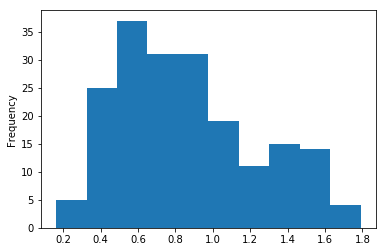
# determine periods under quasi-neutral conditions
limit_neutral = 0.01
ind_neutral = ser_zL.between(-limit_neutral, limit_neutral)
df_val.loc[ind_neutral, 'USTAR'].plot.hist()

[15]:

<matplotlib.axes._subplots.AxesSubplot at 0x1158fd940>

1.4.2.4. calculate roughness length \(z_0\) and zero plane displacement \(d\)¶

1.4.2.4.1. theoretical basis¶

We will employ the followng equation in our calculations:

\[\bar{u}(z)=\frac{u_{*}}{k} \ln \left[\frac{(z-d)}{z_{0}}\right]\]

where \(\bar{u}(z)\) is the measured wind speed at a height \(z\), \(u_{*}\) the friction velocity, \(d\) the zero-plane displacement, \(k\) the von Karman’s constant (a value of 0.4 used in the following calculation).

1.4.2.4.2. calculation¶

We will use scipy.optimize.curve_fit to determine the parameters \(z_0\) and \(d\) in the model above.

[16]:

from scipy.optimize import curve_fit

To use curve_fit, we need to define a function repensenting the model above:

[17]:

def func_uz(ustar, z0):
    z = z_meas
    d = 0.7 * h_sfc
    k = 0.4
    uz = ustar / k * np.log((z - d) / z0)
    return uz

[18]:

# choose the necessary variables
df_sel = df_val.loc[ind_neutral, ['WS', 'USTAR']].dropna()

[19]:

# set up input data for curve fitting
ser_ustar = df_sel.USTAR
ser_ws = df_sel.WS
# use `curve_fit` to get parameters of interest
z0_fit, _ = curve_fit(func_uz, ser_ustar, ser_ws, bounds=[(0), (np.inf)])

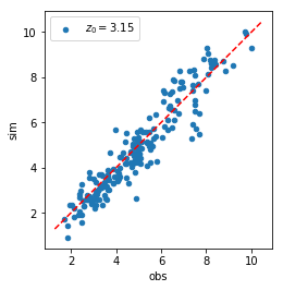
[20]:

# examine the results
res_fit = func_uz(ser_ustar, z0_fit).rename('sim')
res_obs = ser_ws.copy().rename('obs')
df_comp = pd.concat([res_obs, res_fit], axis=1)
ax = df_comp.plot.scatter(x='obs', y='sim', label=f'$z_0=${z0_fit[0]:.2f}')
lim = ax.get_xlim()
ax.plot(lim, lim, color='r', linestyle='--')
ax.set_aspect('equal')

[20]:

[<matplotlib.lines.Line2D at 0x127a4a048>]

1.4.2.4.3. Calculate aerodynamic resistance \(r_a\)¶

1.4.2.4.3.1. write down the equation used for this calculation¶

equation with explanations of symbol:

\[equation\ here\]

1.4.2.4.3.2. calculation¶

[21]:

# calculation code

1.4.2.4.4. examination of variability¶

[22]:

# calculation code