Quickstart of SuPy
This quickstart demonstrates the essential and simplest workflow of supy in SUEWS simulation:
More advanced use of supy are available in the tutorials
Before start, we need to load the following necessary packages.
[1]:
import supy as sp
import pandas as pd
import numpy as np
from pathlib import Path
%matplotlib inline
Load SUEWS input files
First, a path to SUEWS RunControl.nml should be specified, which will direct supy to locate input files.
[2]:
path_runcontrol=Path('../sample_run')/'RunControl.nml'
Model configuration
We call sp.init_supy_df to initialise a SUEWS simulation and get two pandas objects (note: the following names CAN be customised and are NOT fixed to the examples shown here):
df_state_init: a DataFrame for grid-specific settings
Once loaded in, these objects CAN be modified and reused for conducting simulations that differ from the one configured via input files under the above dir_start.
[3]:
df_state_init = sp.init_supy_df(path_runcontrol)
A sample df_state_init looks below (note that .T is used here to a nicer tableform view):
[5]:
df_state_init.filter(like='method').T
[5]:
| grid | 1 | |
|---|---|---|
| var | ind_dim | |
| aerodynamicresistancemethod | 0 | 2 |
| evapmethod | 0 | 2 |
| disaggmethod | 0 | 1 |
| disaggmethodestm | 0 | 1 |
| emissionsmethod | 0 | 2 |
| netradiationmethod | 0 | 3 |
| raindisaggmethod | 0 | 100 |
| roughlenheatmethod | 0 | 2 |
| roughlenmommethod | 0 | 2 |
| smdmethod | 0 | 0 |
| stabilitymethod | 0 | 3 |
| storageheatmethod | 0 | 1 |
| waterusemethod | 0 | 0 |
Meteorological forcing
Following the convention of SUEWS, supy loads meteorological forcing (met-forcing) files at the grid level.
Note:
If `multiplemetfiles = 0` (i.e., all grids use the same met-forcing file) is set in `ser_mod_cfg`, the `grid` argument takes NO effect and is ignored by `supy`.
[6]:
grid = df_state_init.index[0]
df_forcing = sp.load_forcing_grid(path_runcontrol, grid)
Run SUEWS simulations
Once met-forcing (via df_forcing) and initial conditions (via df_state_init) are loaded in, we call sp.run_supy to conduct a SUEWS simulation, which will return two pandas DataFrames: df_output and df_state.
[7]:
df_output, df_state = sp.run_supy(df_forcing, df_state_init)
df_output
df_output is an ensemble output collection of major SUEWS output groups, including:
* SUEWS: the essential SUEWS output variables
* DailyState: variables of daily state information
* snow: snow output variables (effective when `snowuse = 1` set in `ser_mod_cfg`)
* ESTM: ESTM output variables (not implemented yet)
[8]:
df_output.columns.levels[0]
[8]:
Index(['DailyState', 'ESTM', 'SUEWS', 'snow'], dtype='object', name='group')
df_state
df_state is a DataFrame for holding:
- all model states if
save_stateis set toTruewhen callingsp.run_supyandsupymay run significantly slower for a large simulation; - or, only the final state if
save_stateis set toFalse(the default setting) in which modesupyhas a similar performance as the standalone compiled SUEWS executable.
Entries in df_state have the same data structure as df_state_init and can thus be used for other SUEWS simulations staring at the timestamp as in df_state.
[9]:
df_state.T
[9]:
| grid | 1 | ||
|---|---|---|---|
| datetime | 2012-01-01 00:30:00 | 2012-12-31 23:35:00 | |
| var | ind_dim | ||
| aerodynamicresistancemethod | 0 | 2.00 | 2.00 |
| ah_min | (0,) | 15.00 | 15.00 |
| (1,) | 15.00 | 15.00 | |
| ah_slope_cooling | (0,) | 2.70 | 2.70 |
| (1,) | 2.70 | 2.70 | |
| ah_slope_heating | (0,) | 2.70 | 2.70 |
| (1,) | 2.70 | 2.70 | |
| ahprof_24hr | (0, 0) | 0.57 | 0.57 |
| (0, 1) | 0.65 | 0.65 | |
| (1, 0) | 0.45 | 0.45 | |
| (1, 1) | 0.49 | 0.49 | |
| (2, 0) | 0.43 | 0.43 | |
| (2, 1) | 0.46 | 0.46 | |
| (3, 0) | 0.40 | 0.40 | |
| (3, 1) | 0.47 | 0.47 | |
| (4, 0) | 0.40 | 0.40 | |
| (4, 1) | 0.47 | 0.47 | |
| (5, 0) | 0.45 | 0.45 | |
| (5, 1) | 0.53 | 0.53 | |
| (6, 0) | 0.71 | 0.71 | |
| (6, 1) | 0.70 | 0.70 | |
| (7, 0) | 1.20 | 1.20 | |
| (7, 1) | 1.13 | 1.13 | |
| (8, 0) | 1.44 | 1.44 | |
| (8, 1) | 1.37 | 1.37 | |
| (9, 0) | 1.29 | 1.29 | |
| (9, 1) | 1.37 | 1.37 | |
| (10, 0) | 1.28 | 1.28 | |
| (10, 1) | 1.30 | 1.30 | |
| (11, 0) | 1.31 | 1.31 | |
| ... | ... | ... | ... |
| wuprofm_24hr | (11, 0) | -999.00 | -999.00 |
| (11, 1) | -999.00 | -999.00 | |
| (12, 0) | -999.00 | -999.00 | |
| (12, 1) | -999.00 | -999.00 | |
| (13, 0) | -999.00 | -999.00 | |
| (13, 1) | -999.00 | -999.00 | |
| (14, 0) | -999.00 | -999.00 | |
| (14, 1) | -999.00 | -999.00 | |
| (15, 0) | -999.00 | -999.00 | |
| (15, 1) | -999.00 | -999.00 | |
| (16, 0) | -999.00 | -999.00 | |
| (16, 1) | -999.00 | -999.00 | |
| (17, 0) | -999.00 | -999.00 | |
| (17, 1) | -999.00 | -999.00 | |
| (18, 0) | -999.00 | -999.00 | |
| (18, 1) | -999.00 | -999.00 | |
| (19, 0) | -999.00 | -999.00 | |
| (19, 1) | -999.00 | -999.00 | |
| (20, 0) | -999.00 | -999.00 | |
| (20, 1) | -999.00 | -999.00 | |
| (21, 0) | -999.00 | -999.00 | |
| (21, 1) | -999.00 | -999.00 | |
| (22, 0) | -999.00 | -999.00 | |
| (22, 1) | -999.00 | -999.00 | |
| (23, 0) | -999.00 | -999.00 | |
| (23, 1) | -999.00 | -999.00 | |
| year | 0 | 2012.00 | 2012.00 |
| z | 0 | 10.00 | 10.00 |
| z0m_in | 0 | 0.01 | 0.01 |
| zdm_in | 0 | 0.20 | 0.20 |
1281 rows × 2 columns
Examine SUEWS results
Thanks to the functionality inherited from pandas and other packages under the PyData stack, compared with the standard SUEWS simulation workflow, supy enables more convenient examination of SUEWS results by statistics calculation, resampling, plotting (and many more).
Ouptut structure
df_output is organised with MultiIndex (grid,timestamp) and (group,varaible) as index and columns, respectively.
[10]:
df_output.head()
[10]:
| group | SUEWS | ... | DailyState | |||||||||||||||||||
|---|---|---|---|---|---|---|---|---|---|---|---|---|---|---|---|---|---|---|---|---|---|---|
| var | Kdown | Kup | Ldown | Lup | Tsurf | QN | QF | QS | QH | QE | ... | DSnowPvd | DSnowBldgs | DSnowEveTr | DSnowDecTr | DSnowGrass | DSnowBSoil | DSnowWater | a1 | a2 | a3 | |
| grid | datetime | |||||||||||||||||||||
| 1 | 2012-01-01 00:30:00 | 0.153333 | 0.0184 | 344.310184 | 372.270369 | 11.775916 | -27.825251 | 0.0 | -59.305405 | 31.480154 | 0.0 | ... | NaN | NaN | NaN | NaN | NaN | NaN | NaN | NaN | NaN | NaN |
| 2012-01-01 00:35:00 | 0.153333 | 0.0184 | 344.310184 | 372.270369 | 11.775916 | -27.825251 | 0.0 | -59.305405 | 31.480154 | 0.0 | ... | NaN | NaN | NaN | NaN | NaN | NaN | NaN | NaN | NaN | NaN | |
| 2012-01-01 00:40:00 | 0.140000 | 0.0168 | 344.343664 | 372.308487 | 11.783227 | -27.841623 | 0.0 | -59.318765 | 31.477141 | 0.0 | ... | NaN | NaN | NaN | NaN | NaN | NaN | NaN | NaN | NaN | NaN | |
| 2012-01-01 00:45:00 | 0.126667 | 0.0152 | 344.377146 | 372.346609 | 11.790539 | -27.857996 | 0.0 | -59.332125 | 31.474129 | 0.0 | ... | NaN | NaN | NaN | NaN | NaN | NaN | NaN | NaN | NaN | NaN | |
| 2012-01-01 00:50:00 | 0.113333 | 0.0136 | 344.410631 | 372.384734 | 11.797850 | -27.874370 | 0.0 | -59.345486 | 31.471116 | 0.0 | ... | NaN | NaN | NaN | NaN | NaN | NaN | NaN | NaN | NaN | NaN | |
5 rows × 245 columns
Here we demonstrate several typical scenarios for SUEWS results examination.
The essential SUEWS output collection is extracted as a separate variable for easier processing in the following sections. More advanced slicing techniques are available in pandas documentation.
[11]:
df_output_suews=df_output['SUEWS']
Statistics Calculation
We can use .describe() method for a quick overview of the key surface energy balance budgets.
[12]:
df_output_suews.loc[:,['QN','QS','QH','QE','QF']].describe()
[12]:
| var | QN | QS | QH | QE | QF |
|---|---|---|---|---|---|
| count | 105397.000000 | 105397.000000 | 105397.000000 | 105397.000000 | 105397.0 |
| mean | 43.088982 | -1.439391 | 39.086828 | 5.441544 | 0.0 |
| std | 136.465193 | 111.355598 | 26.836115 | 10.734807 | 0.0 |
| min | -85.761254 | -106.581183 | -47.952449 | 0.000000 | 0.0 |
| 25% | -41.724491 | -70.647184 | 25.932217 | 0.000000 | 0.0 |
| 50% | -25.247367 | -57.201851 | 29.431719 | 0.000000 | 0.0 |
| 75% | 78.333777 | 27.320362 | 45.689971 | 5.911592 | 0.0 |
| max | 698.440633 | 533.327557 | 165.113077 | 125.956522 | 0.0 |
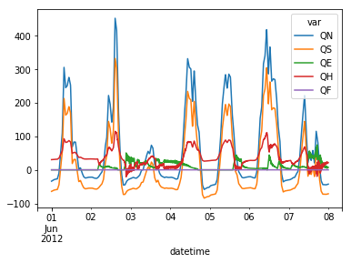
Plotting
Plotting is very straightforward via the .plot method bounded with pandas objects.
[19]:
df_output_suews.loc[1].loc[
    '2012 6 1':'2012 6 7',
    ['QN','QS','QE','QH','QF']
].plot()
[19]:
<matplotlib.axes._subplots.AxesSubplot at 0x12289eac8>
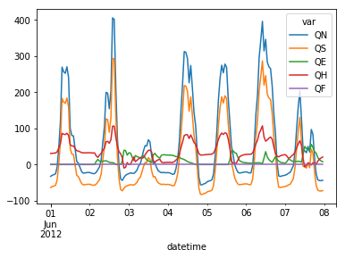
Resampling
The suggested runtime/simulation frequency of SUEWS is 300 s, which usually results a large output and may be over-weighted for storage. To slim down the output size, we can resample the default output.
[14]:
df_output_suews_rsmp=df_output_suews.loc[1].resample('1h').mean()
[15]:
df_output_suews_rsmp.loc[
    '2012 6 1':'2012 6 7',
    ['QN','QS','QE','QH','QF']].plot()
[15]:
<matplotlib.axes._subplots.AxesSubplot at 0x11ea2d400>
The resampled output can be outputed for a smaller file.
[16]:
df_output_suews_rsmp.to_csv('suews_1h.txt',
                            sep='\t',
                            float_format='%8.2f',
                            na_rep=-999)
For a justified format, we use the to_string for better format controlling and write the formatted string out to a file.
[17]:
str_out=df_output_suews_rsmp.to_string(
    float_format='%8.2f',
    na_rep='-999',
    justify='right')
with open('suews_sample.txt','w') as file_out:
    print(str_out,file=file_out)