1. Evaporation, Penman Monteith
Dr Ting Sun (ting.sun@reading.ac.uk)
11 Oct 2018
1.1. Measuring Humidity Fluxes
1.1.1. (open-path) Infra-Red Gas Analyzer (IRGA)
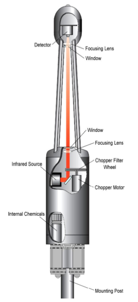
1.1.1.1. How does it work?
IDGA measures CO2 and water vapor densities in air based on non-dispersive infrared spectroscopy:
- Infrared radiation is transmitted first through temperature-controlled optical filters and then an open sample path to a thermally regulated detector
- Some of the infrared radiation is absorbed by CO2 and water vapor in the sample path
- Gas densities are computed from the ratio of absorbed radiation to a reference.
- Wavelength at which different atmospheric gases absorb infrared radiation
| content | wave length |
|---|---|
| Water Vapour | 2.59 µm and 2.40 µm |
| Carbon Dioxide | 4.26 µm and 3.95 µm |
1.2. Moisture Flux, Evaporation and Latent Heat
| symbol | meaning | unit |
|---|---|---|
| \(\overline{q}\) | Specific Humidity | \(\mathrm{kg \ {kg}^{-1}}\) |
| \(\overline{w'q'}\) | Moisture Flux | \(\mathrm{kg \ {kg}^{-1}\ {m}^{-2}\ {m}^{-1}}\) |
| \(Q_E\) or \(\lambda E\) | Latent heat of vaporization | \(\mathrm{W\ {m}^{-2}}\) |
| \(E\) | Evaporation | \(\mathrm{mm \ {d}^{-1}}\) |
1.2.1. approximations
| water equivalent | energy equivalent |
|---|---|
| \(\mathrm{1\ mm \ {d}^{-1}}\) | \(\mathrm{28.3\ W \ {m}^{-2}}\) |
| \(\mathrm{1\ mm \ {h}^{-1}}\) | \(\mathrm{680\ W \ {m}^{-2}}\) |
Note:
- these approximations are valid at \(20\ \mathrm{°C}\)
- they change with \(L_v\), \(\rho_w\)
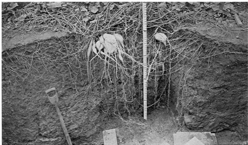
1.3. How to model evaporation with easily observed measurements at one height?
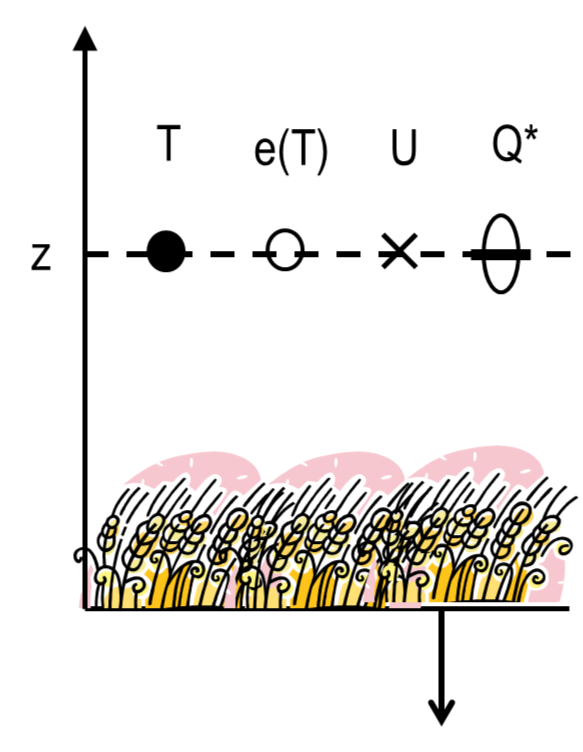
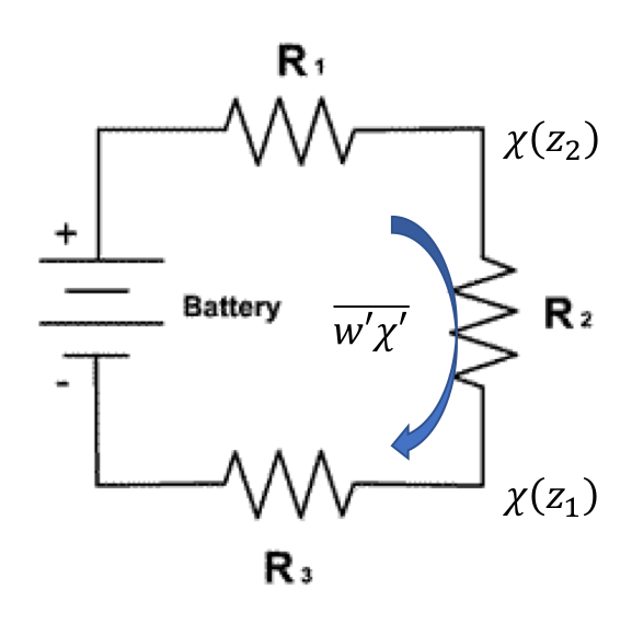
1.3.1. Use of Resistances
| Electrical Analogy | Resistance network for a surface scheme |
|---|---|
 |
 |
1.4. The Combination Equation
sensible heat flux
\[Q_H=\rho c_p \frac{T-T_0}{r_h}\]latent heat flux
\[Q_E=\frac{L_v}{R_v T} \frac{e-e_0}{r_v}=\frac{\rho c_p}{\gamma_*}\frac{e-e_0}{r_h}\]Linearize saturated vapour pressure
\[e_0=e_s(T_0)=e_s(T)-s(T-T_0)\]
where \(s=\frac{d e_s}{dT}\)
1.5. Derivation of Penman Equation
1.5.1. Goal: To obtain an expression of \(Q_E\) as a function of
- available energy
bear in mind the surface energy balance \(Q^*-Q_G=Q_H+Q_E\) by neglecting: 1) advection heat \(Q_{\text{adv}}\); and 2) anthropogenic heat: \(Q_F\) (e.g. in an urban environment).
- surface level meteorological factors:
- air temperature \(T\)
- air humidity in vapour pressure \(e(T)\)
1.5.2. Derivation using sympy
[1]:
from sympy import *
init_printing()
[2]:
qh,qe,qn,qg=symbols('Q_H,Q_E,Q^*,Q_G')
t,t0,et,e0,e,s=symbols('T,T_0,e_T,e_0,e,s')
rho,gms,cp,rh,rv=symbols(r'\rho,\gamma_*,c_p,r_h,r_v')
[3]:
sol=solve([
    qn-qg-qh-qe,
    qe-(rho*cp/gms)*((e-e0)/rh),
    qh-(rho*cp*(t-t0)/rh),
    e0-et-s*(t-t0)
],
    [qe,qh,e0,t0])
sol_qe=sol.get(qe)
[4]:
qa,de=symbols('Q_a,de')
apart(sol_qe.subs({qn:qa+qg,e:et+de}),qa).subs({qa:qn-qg,de:e-et})
[4]:
1.6. Penman (1948) Equation
Penman equation:
\[Q_E=L_VE=\frac{s \left(Q^{*} - Q_{G}\right)}{- \gamma_* + s}- \frac{\rho c_{p} \left(e - e_{T}\right)}{- \gamma_* r_{h} + r_{h} s}\]Advantage:
- Estimation of evaporation from simple measurements
- Using measurements at low heights: can neglect stability dependence of resistance
- Approximate resistance for heat transfer by the aerodynamic resistance
Remaing Challenge:
- How to determine \(\gamma_*=\gamma \frac{r_v}{r_h}\)?
1.7. Wind’s Influence on Evaporation
1.7.1. Modified Penman-Monteith equation:
where
| symbol | meaning | unit |
|---|---|---|
| \(s\) | slope of \(e_s(T_a)\) | \(\mathrm{Pa \ {°C}^{-1}}\) |
| \(c_p\) | heat capacity of air | \(\mathrm{J \ {m}^{-3} \ {°C}^{-1}}\) |
| \(\rho\) | density of air | \(\mathrm{kg \ {m}^{-3} }\) |
| \(\gamma\) | psychometric constant | \(\mathrm{Pa \ {°C}^{-1}}\) |
| \(V\) | vapour pressure deficit of air | \(\mathrm{Pa}\) |
| \(r_a\) | aerodynamic resistance | \(\mathrm{s \ m^{-1}}\) |
| \(r_s\) | surface resistance | \(\mathrm{s \ m^{-1}}\) |
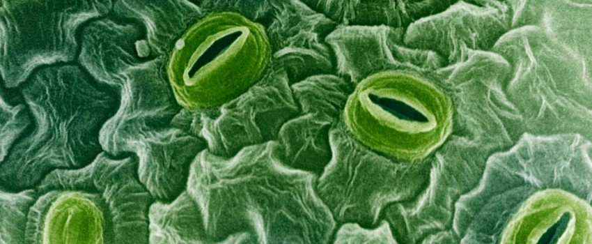
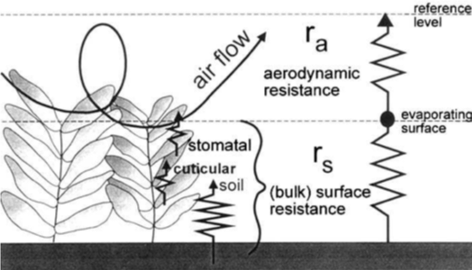
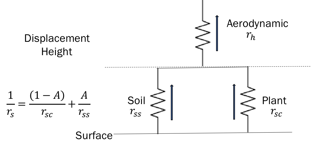
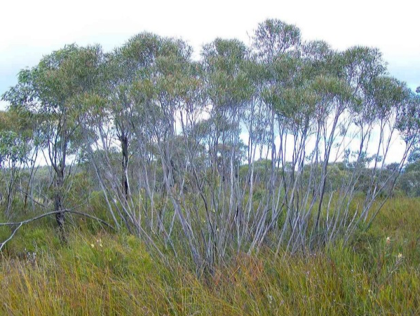
1.8. Surface Transfers as Electrical Circuits
Total resistance for vapour:
\[{r_v}={r_s}+{r_h}\]
| resistance network | real-world canopy |
|---|---|
 |
 |
1.9. Exercises
Manual derivation of Penman (1948) equation.
The Penman Monteith equation provides one method to calculate the components of the surface energy balance. It assumes energy balance closure at each model time step (see the notes along with Assignment 1). Evaluate the performance of the PM calculations using the EC data (e.g. \(Q_H\) and \(Q_E\), \(\beta\)).
Calculate the canopy resistance from the EC and other data (this can be back-calculated). How do these values compare to the literature/textbooks?
note: You will need dry conditions (e.g. 12 h since rain – depending on time of day) and solar radiation for the calculations (e.g. \(Q^* \gt \mathrm{20\ W \ {m}^{-2}}\))