This page was generated from docs/tutorials/DataAnalysis_BLM.ipynb. Interactive online version: Slideshow:

Data Analysis Tutorial for BLM

Dr Ting Sun (ting.sun@reading.ac.uk)

2018 Autumn

Basic Workflow

• Import (and pre-process)
• Analyse
• Deliver

Tools

Essential:

• numpy: a fundamental package for scientific computing
• pandas: a 1D (Series) and 2D (DataFrame, aka tabular data) data analysis package
• matplotlib: a plotting package for producing publication quality figures

Advanced:

• seaborn: a matploblib-based high-level plotting package
• xarray: the high-dimensional “pandas”
• dask: the parallel “pandas”

Example 1: Evaporation analysis using Penman equation

Aim

1. To obtain the essential skills in data analysis
2. To understand the nature of the Penman equation

Questions

1. How to use the Penman equation to estimate evaporation?
   • what are the parameters that need to be prescribed?
   • what are the input/forcing data you should prepare?
2. Examination of Penman-based results
   • how do we know the accuracy of our estimates? any ‘truth’ data?
   • what indicators should we calculate?
3. Importing the raw data and preprocessing it to do your own analysis?
   • is it time-aware?
   • any gaps? to fill or not? if needed, how to fill the gaps?
4. What are extrinsic and intrinsic determinants of estimated evaporation based on Penman equation?
   • what parameters are set by us?
   • what forcing data are used?
   • what will happen if we perturb/adjust some of/all the above factors? and why? any physical explanations?

Import

load necessary packages

import pandas as pd
import numpy as np
import matplotlib.pyplot as plt
import seaborn as sns
%matplotlib inline

import raw data

data_raw = pd.read_csv('../data/PM_rawdata.csv', header=[0, 1]).dropna(how='all')
data_raw.head().T.head()

		0	1	2	3	4
TimeStamp	UTC	2.01509e+07	2.01509e+07	2.01509e+07	2.01509e+07	2.01509e+07
Time	hhmm	5	10	15	20	25
Td	deg C	5.89	5.71	5.67	5.58	5.51
Tw	deg C	5.66	5.61	5.51	5.38	5.4
RH	%	98.3	98.9	98.7	98.1	98.7

DateTime-related pre-processing

# generate correct timestamps
def parse_dt(date, time):
    date = pd.to_datetime(int(date), format='%Y%m%d')
    time_str = str(int(time)).zfill(4)
    timedelta_str = time_str[:2]+'h'+time_str[2:]+'m'
    timedelta = pd.Timedelta(timedelta_str)
    dt = date+timedelta
    return dt


ser_dt = data_raw.iloc[:, [0, 1]].apply(lambda x: parse_dt(*x), axis=1)

# add the `datetime` column
data_raw['datetime'] = ser_dt

# set a new index series to `data_PM` used for the following analysis
data_PM = data_raw.iloc[:, 2:].set_index('datetime')

Analyse

Modified Penman-Monteith equation:

\[Q_E=L_VE=\frac{s \left(Q^{*} - Q_{G}\right)}{s+ \gamma \left( 1+r_s/r_a \right)}+ \frac{\rho c_{p} \left(e_{T} - e\right)/r_a}{s+ \gamma \left( 1+r_s/r_a \right)}\]

Parameters:

factors that are NOT changing during one model run:

symbol	unit	meaning	default value
\(\gamma\)	\(\mathrm{Pa\ {°C}^{-1}}\)	psychometric constant	0.67
\(\rho\)	\(\mathrm{kg\ {m}^{-3} }\)	density of air	1.2
\(c_p\)	\(\mathrm{J\ {m}^{-3} \ {°C}^{-1}}\)	heat capacity of air	1004
\(r_s\)	\(\mathrm{s\ m^{-1}}\)	surface resistance	60

Forcing data

factors that should be provided at each time step during one model run:

symbol	unit	meaning
\(Q^{*}\)	\(\mathrm{W\ m^{-2}}\)	net wall-wave radiation
\(Q_{G}\)	\(\mathrm{W\ m^{-2}}\)	ground heat flux
\(e\)	\(\mathrm{Pa}\)	vapour pressure
\(T_a\)	\(\mathrm{°C}\)	air temperature
\(U\)	\(\mathrm{m\ s^{-1}}\)	wind speed

Intermediate states

factors that are calculated based on forcing data and parameters but are NOT the main outputs

symbol	unit	meaning
\(e_T\)	\(\mathrm{Pa}\)	saturation evaporation pressure
\({s}\)	\(\mathrm{Pa \ {°C}^{-1}}\)	slope of \(e_s(T_a)\)
\(r_a\)	\(\mathrm{s\ m^{-1}}\)	aerodynamic resistance

Implementation: calc_PM

• auxiliary functions: we use atmos as the basic utility.
  • esat(Ta): saturation vapour pressure at \(T_a\)
  • s(Ta): saturation vapour pressure slope at \(T_a\)
  • ra(U): aerodynamic resistance at \(U\)

from atmos import calculate as atm_calc


# saturation vapour pressure in [hPa] at Ta
def esat_hPa(Ta_K):
    return atm_calc('es', T=Ta_K)/100


# saturation vapour pressure in [hPa K-1] slope at Ta
def s_esat_hPaKn1(Ta_K):
    dTa_K = 0.001
    d_esat = (esat_hPa(Ta_K)-esat_hPa(Ta_K-dTa_K))
    return d_esat/dTa_K


# aerodynamic resistance in [s m-1] at U
def res_air_smn1(U, z_Ta=1.5, z_U=3, z0=0.01, k=0.4):
    ustar = k*U/np.log(z_U/z0)
    res_air = np.log(z_Ta/z0)/(ustar*k)
    return res_air

• calc_PM

def calc_PM(Qn, QG, e, Ta, U, rho=1.2, cp=1004, gamma=0.67, rs=60, z_Ta=1.5, z_U=3, z0=0.01, k=0.4):
    Ta_K = Ta+273.15
#   slope
    s = s_esat_hPaKn1(Ta_K)
#   aerodynamic resistance
    ra = res_air_smn1(U, z_Ta, z_U, z0, k)
#   numerator of PM equation
    num_PM = s*(Qn-QG)+rho*cp*(esat_hPa(Ta_K)-e)/ra
#   denominator of PM equation
    denom_PM = s+gamma*(1+rs/ra)
#   QE from PM equation
    qe = num_PM/denom_PM
    return qe

Qn = data_PM.loc[:, 'Rn'].iloc[:, 0].rename('Qn')
QG = data_PM.loc[:, 'G'].iloc[:, 0].rename('QG')
e = data_PM.loc[:, 'VP_der'].iloc[:, 0]
Ta = data_PM.loc[:, 'Td'].iloc[:, 0]
U = data_PM.loc[:, 'U10'].iloc[:, 0]
QE = calc_PM(Qn, QG, e, Ta, U).rename('QE')
QH = (Qn-QG-QE).rename('QH')

Examine the SEB components

df_SEB=pd.DataFrame([Qn,QG,QE,QH]).T
df_SEB.plot()

<matplotlib.axes._subplots.AxesSubplot at 0x115066358>

Exploration

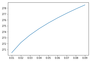
Impacts of measurement height of wind speed z_U

ser_z_U=pd.Series(np.arange(3,10,1))

df_QE_zU=pd.DataFrame({x:calc_PM(Qn, QG, e, Ta, U, z_U=x) for _,x in ser_z_U.iteritems()})

df_QE_zU.max().plot()

<matplotlib.axes._subplots.AxesSubplot at 0x117dd9cf8>

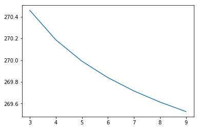
Impacts of measurement height of surface roughness length z0

ser_z0=pd.Series(np.arange(0.01,0.1,0.01))

df_QE_z0=pd.DataFrame({x:calc_PM(Qn, QG, e, Ta, U, z0=x) for _,x in ser_z0.iteritems()})

# df_QE_z0.mean().plot.barh()

df_QE_z0.max().plot()

<matplotlib.axes._subplots.AxesSubplot at 0x117eb4240>

Example 2: Wind and Temperature Profile

Basics about wind and temperature profiles

neutral conditions

The variation of mean wind speed \(\bar{u}\) with height \(z\) (in surface layer, above the RSL) above an aerodynamically rough surface can be represented by a logarithmic relation:The variation of mean wind speed \(\bar{u}\) with height \(z\) (in surface layer, above the RSL) above an aerodynamically rough surface can be represented by a logarithmic relation:

\[\bar{u}=\frac{u_*}{k} \ln \left[ \frac{z-d}{z_0} \right]\]

where where \(u_*\) is the friction velocity (\(u_*^2=-\overline{u'w'}\)) (rate of vertical transfer by turbulence of horizontal momentum per unit mass of air), \(z_0\) is the roughness length of the surface for momentum, \(d\) is the zero-plane displacement and \(k\) is von Karman’s constant (0.4).

The logarithmic law is strictly valid only in neutral conditions, i.e. when the effect of buoyancy on turbulence is small compared to the effect of wind shear. In such conditions, the temperature profile in the surface layer will be close to adiabatic (i.e. \(dT/dz = –9.8 \textrm{ K km}^{-1}\) or potential temperature is constant with height). When the sensible heat flux is significantly different from zero, Monin-Obukhov theory must be used.

non-neutral conditions

Modifications to the logarithmic profile are required in conditions of non-neutral stability, using the results of Monin-Obukhov theory. This theory of the surface layer derives relations between the vertical variation of wind speed \(u(z)\) and potential temperature \(\theta(z)\) (which approximates the measured temperature \(T\) close to the surface), the scaling factors for momentum and temperature, \(u_*\) and \(T_*\), and the Monin-Obukhov stability parameter,

\[\zeta=\frac{z'}{L}=\frac{k (z-d)}{u_*^3}\frac{g}{\theta_0}\frac{Q_H}{\rho c_p}\]

where \(L\) is the Obukhov length and \(z' = z - d\).

NB: the surface temperature \(\theta_0\) is an absolute temperature (units: K).

The logarithmic profile relation can be rewritten for wind speed to include the stability corrections:

\[\bar{u}(z)=\frac{u_*}{k} \left[ \ln \left( \frac{z-d}{z_0} \right) -\Psi_m \left( \frac{z-d}{L} \right) + \Psi_m \left( \frac{z_0}{L} \right) \right]\]

and similarly for potential temperature:

\[\bar{\theta}(z)=\theta_0+\frac{T_*}{k} \left[ \ln \left( \frac{z-d}{z_{0h}} \right) -\Psi_h \left( \frac{z-d}{L} \right) + \Psi_h \left( \frac{z_{0h}}{L} \right) \right]\]

where the turbulent temperature scale is given by

\[T_*=-\overline{w'T'}/u_*=-Q_H/\left(\rho c_p u_*\right)\]

\(\Psi_m\) is the stability correction function for momentum and \(\Psi_h\) is the stability correction function for heat. Note that both \(T_*\) and \(z’/L\) have the opposite sign to \(Q_H\) (which is positive in unstable conditions and negative in stable conditions).

stability correction functions

The above mentioned stability corretion functions are formulated based on the Monin-Obukhov similarity theory (MOST) and their actual forms must be determined theoretically (e.g., Katul et al. (2011), Li et al. (2012)) or empirically (e.g., Högström (1988)).

One example by Kondo (1975) is as follows:

• unstable conditions:

\[\Psi_{h} = 2 \ln \left[ \frac{1+(1-16\zeta)^{1/2}}{2} \right]\]

\[\Psi_{m} = 0.6\Psi_{h}\]

• stable conditions:

\[\Psi_{m} = \Psi_{h}=-6 \ln (1+\zeta)\]

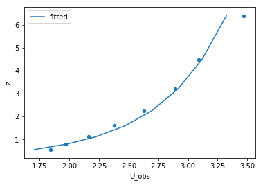
Unstable case

import raw data

# data_raw=pd.read_csv('WP_PM_rawdata.csv',header=0,skiprows=[1]).dropna(how='all')
data_raw = pd.read_csv('../data/WP_unstable_rawdata.csv', header=[0, 1]).dropna(how='all')
data_raw

	z	U_obs	T_obs
	(m)	(m/s)	(C)
0	0.56	1.84	24.91
1	0.80	1.97	NaN
2	1.12	2.16	24.39
3	1.60	2.38	NaN
4	2.24	2.63	23.76
5	3.20	2.89	NaN
6	4.48	3.09	23.90
7	6.40	3.47	NaN

implement the stability correction function

# Psi for momentum under unstable condition
def Psi_m_unstable(z_d, L):
    z_L = z_d/L
    Psi_m = 0.6*(2)*np.log((1+(1-16*z_L)**0.5)/2)
    return Psi_m


# wind profile function
def func_u_z(z, u_star, z0, d=0.01, L=-2.1998, k=0.4):
    crt = np.log((z-d)/z0)-Psi_m_unstable(z-d, L)+Psi_m_unstable(z0, L)
    fit_u_z = u_star/k * crt
    return fit_u_z


# form for fitting
def func_fit_u_z(z, u_star, z0):
    return func_u_z(z, u_star, z0)

fit curve by scipy.optimize

from scipy import optimize
params, params_covariance = optimize.curve_fit(func_fit_u_z,
                                               data_raw.z.values.flatten(),
                                               data_raw.U_obs.values.flatten())
pd.Series(params,index=['u_star','z0']).to_frame().T

	u_star	z0
0	0.468304	0.083681

examine the fitted curve

# clean the labels
data_fit = data_raw.copy()[['z', 'U_obs']]
data_fit.columns = data_fit.columns.droplevel(1)

# data_fit
data_fit['U_fit'] = func_fit_u_z(data_fit.z, *params)
data_fit

	z	U_obs	U_fit
0	0.56	1.84	1.705202
1	0.80	1.97	1.980512
2	1.12	2.16	2.225307
3	1.60	2.38	2.470980
4	2.24	2.63	2.691432
5	3.20	2.89	2.914837
6	4.48	3.09	3.117291
7	6.40	3.47	3.324439

ax = data_fit.plot.line(x='U_fit', y='z', label='fitted')
data_fit.plot.scatter(ax=ax, x='U_obs', y='z')

<matplotlib.axes._subplots.AxesSubplot at 0x115bb3320>

exercise: fit the temperature profile

# what stability corrections should be used for temperature profiles?

# what is the fitting function for temperature profiles?

Stable case

exercise:

# adapt the above analysis under unstable condition to the stable condition

• wind speed profile

# adapt the above analysis under unstable condition to the stable condition

• temperature profile

# adapt the above analysis under unstable condition to the stable condition

Exploration: impacts of surface roughness on the profiles

Think about:

• How is surface roughness accounted for in the calculation of the above profiles?
• Do wind directions matter in the above calculations?

# write your code here to answer the above questions